last change: 2021-10-24
Arithmetic Compression / Arithmetic Coding
Introduction
1. Data Preparation
1.0. Orignal
1.1. Subtract Green Transform
1.2. Channel-Wise Deltas
1.3. Zigzag Encoding
2. Compression
2.1. Arithmetic Encoding
2.2. Heatmap of Bits per Symbol (Absolute)
2.3. Heatmap of Bits per Symbol (Brightened)
Preface
This article is just for fun. Arithmetic compression is outdated. Its compression ratio is excellent, but the throughput is rather low. Therefor, compression algorithms based on ANS (asymmetric numeral systems) are the state of the art in entropy coding. Furthermore, ANS was always free to use, unlike arithmetic compression, which was patented and not free to use for many years.
The terms arithmetic compression and arithmetic coding are used synonymously in this article.
Introduction
This article shows results of playing around with arithmetic compression, which is a kind of entropy compression. It's suitable for compressing chains of symbols which have a non-uniform distribution, but appear to be otherwise random. The distribution must be either known at compression start time or it can be discovered during the compression process (adaptive arithmetic compression). Arithmetic compression typically results in smaller sizes than huffman coding, because arithmetic compression combines multiple symbols to one result, thereby using a fractional number of bits per symbol, while huffman coding always uses a rounded-up integer number of bits for every symbol, even if only a fractional number of information is conveied by the symbol.
The code (not published yet) which I wrote for the arithmetic compression is a Java implementation of the pseudocode given in chapter 4 "Arithmetic Coding" of the book Introduction to Data Compression, by Khalid Sayood. In this book, the introduction to chapter 4 starts with the words "In the last chapter we studied the Huffman coding method". What follows is an excellent educational read about how it's possible to design a coding which can encode to even shorter codes than huffman coding as well as stepwise explanations and examples for understanding arithmetic coding, leading up to pseudocode using integer arithmetic for encoding and decoding.
Photos are a nice target for seeing how arithmetic compression works, because it's easy to visualize the required steps.
1. Data Preparation
1.0. Orignal
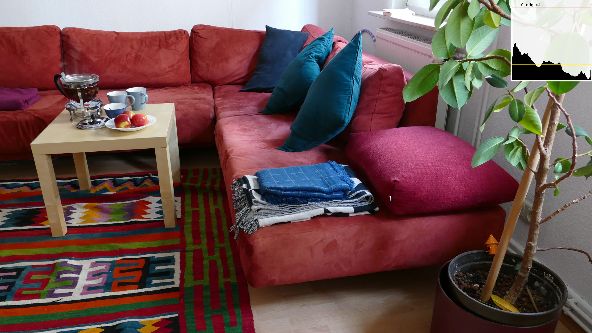
Note that the distribution (= historgram, see upper right corner of the image) of the pixel data already is a non-uniform distribution. However, it can be preprocessed to get it even further away from a uniform distribution (i.e. to make it even more skewed), thus better suited for arithmetic compression. Here we do this by subtracting strongly correlated values from each other and encoding the resulting deltas (= differences) instead of the direct pixel data. We do this in two steps, the first is called the subtract green transform and the second is channel-wise deltas from the previous pixel.
1.1. Subtract Green Transform
for i=0..n-1
    r[i] -= g[i]
    b[i] -= g[i]
 (without histogram)
The subtract green transform, as the name says, subtracts, for every pixel, the amount of green from the red and from the blue channels of the pixel. If the result is negative, an overflow happens (because pixel channel values are unsigned), but this operation is still reversible, so no information is lost and we simply go on with the calculation.
1.2. Channel-Wise Deltas
for i=n-1..1
    r[i] -= r[i-1]
    // ... same for g[i] and b[i]
Again, negative results -1, -2, -3, ..., -128 overflow and end up at byte values 255, 254, 253, ..., 128, so they show up at the right end of the historgram.
 (without histogram)
After this step, we are ready to apply arithmetic compression. However, the histogram doesn't look nice with it's two peaks, so we apply an additional zigzag encoding, which redistributes both peaks to the left of the histogram.
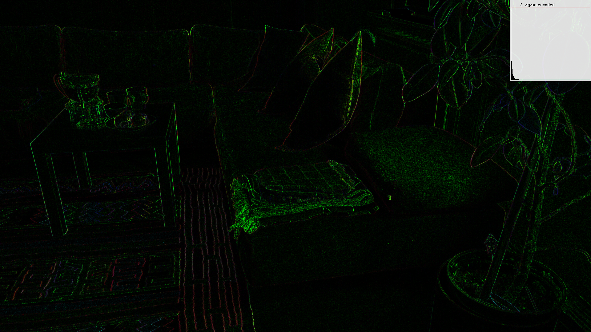
1.3. Zigzag Encoding
The zigzag encoding step is completely useless for arithmetic coding, because arithmetic coding only cares about the individual frequencies of the symbols, but not about the order of the frequency table that you use for encoding. When you leave out the zigzag encoding, the size of the compression output will be just the same. However, I like it more when a distribution looks clean, so I added the zigzag encoding anyways.
for i=0..n-1
    r[i] = (r[i] < 128) ? (r[i] * 2) : ((255 - r[i]) * 2 + 1)
    // ... same for g[i] and b[i]
Lower (positive) values 0..127 get mapped to the even values 0, 2, 4, ..., 254.
Higher (originally negative) values 255..128 get mapped to the odd values 1, 3, 5, ..., 255.
 (without histogram)
2. Compression
2.1. Arithmetic Encoding
The result is expected to be uniformly distributed and significantly shorter
than the original image.
 (without histogram)
The black area is unused memory and it's just there to visualize the amount of memory saved by arithmetic compression. The upper part is the compressed data and it looks fairly uniformly distributed. Just a few more 0's than other values. The displayed histogram is only about the compression result. It doesn't include the black area below.
2.2. Heatmap of Bits per Symbol (Absolute)
Every channel of every pixel is one symbol, which gets encoded individually. The heatmap shows how many bits were written to the stream for each channel of each pixel. This doesn't mean that this one symbol takes up such and such many bits, but usually many bits are written at or closely after regions of high entropy.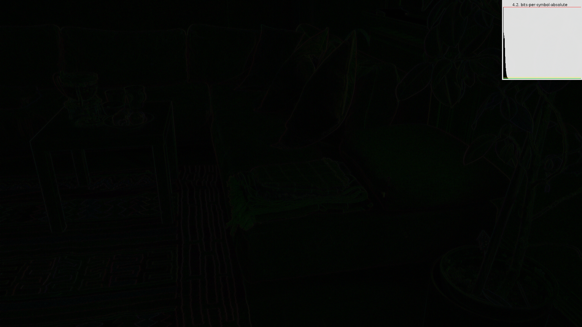 (without histogram)
At first glance, this picture looks like it's completely black, but it's actually just very dark. This absolute heat map is therefor not suitable for spotting anything with the human eye. Next is the same picture, just brightened.
2.3. Heatmap of Bits per Symbol (Brightened)
Like 4.2., but scaled so it's brighter, thus nicer to look at. (without histogram)